How to Collect Data for Binary Logit Model

Daily writing prompt
Share a story about someone who had a positive impact on your life.

By Kavita Dehalwar

Collecting data for a binary logit model involves several key steps, each crucial to ensuring the accuracy and reliability of your analysis. Here’s a detailed guide on how to gather and prepare your data:

1. Define the Objective

Before collecting data, clearly define what you aim to analyze or predict. This definition will guide your decisions on what kind of data to collect and the variables to include. For a binary logit model, you need a binary outcome variable (e.g., pass/fail, yes/no, buy/not buy) and several predictor variables that you hypothesize might influence the outcome.

2. Identify Your Variables

  • Dependent Variable: This should be a binary variable representing two mutually exclusive outcomes.
  • Independent Variables: Choose factors that you believe might predict or influence the dependent variable. These could include demographic information, behavioral data, economic factors, etc.

3. Data Collection Methods

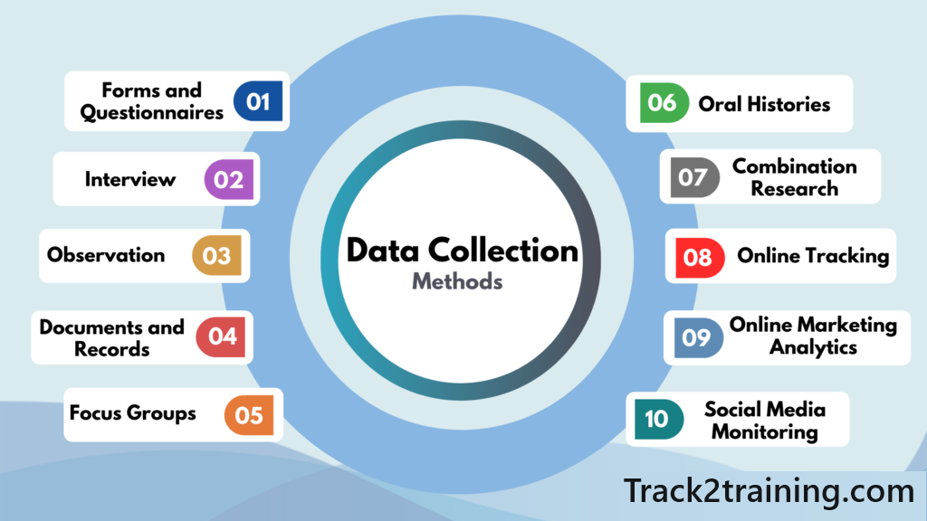
There are several methods you can use to collect data:

  • Surveys and Questionnaires: Useful for gathering qualitative and quantitative data directly from subjects.
  • Experiments: Design an experiment to manipulate predictor variables under controlled conditions and observe the outcomes.
  • Existing Databases: Use data from existing databases or datasets relevant to your research question.
  • Observational Studies: Collect data from observing subjects in natural settings without interference.
  • Administrative Records: Government or organizational records can be a rich source of data.

4. Sampling

Ensure that your sample is representative of the population you intend to study. This can involve:

  • Random Sampling: Every member of the population has an equal chance of being included.
  • Stratified Sampling: The population is divided into subgroups (strata), and random samples are drawn from each stratum.
  • Cluster Sampling: Randomly selecting entire clusters of individuals, where a cluster forms naturally, like geographic areas or institutions.

5. Data Cleaning

Once collected, data often needs to be cleaned and prepared for analysis:

  • Handling Missing Data: Decide how you’ll handle missing values (e.g., imputation, removal).
  • Outlier Detection: Identify and treat outliers as they can skew analysis results.
  • Variable Transformation: You may need to transform variables (e.g., log transformation, categorization) to fit the model requirements or to better capture the nonlinear relationships.
  • Dummy Coding: Convert categorical independent variables into numerical form through dummy coding, especially if they are nominal without an inherent ordering.

6. Data Splitting

If you are also interested in validating the predictive power of your model, you should split your dataset:

  • Training Set: Used to train the model.
  • Test Set: Used to test the model, unseen during the training phase, to evaluate its performance and generalizability.

7. Ethical Considerations

Ensure ethical guidelines are followed, particularly with respect to participant privacy, informed consent, and data security, especially when handling sensitive information.

8. Data Integration

If data is collected from different sources or at different times, integrate it into a consistent format in a single database or spreadsheet. This unified format will simplify the analysis.

9. Preliminary Analysis

Before running the binary logit model, conduct a preliminary analysis to understand the data’s characteristics, including distributions, correlations among variables, and a preliminary check for potential multicollinearity, which might necessitate adjustments in the model.

By following these steps, you can collect robust data that will form a solid foundation for your binary logit model analysis, providing insights into the factors influencing your outcome of interest.

References

Cramer, J. S. (1999). Predictive performance of the binary logit model in unbalanced samples. Journal of the Royal Statistical Society: Series D (The Statistician)48(1), 85-94.

Dehalwar, K., & Sharma, S. N. (2023). Fundamentals of Research Writing and Uses of Research Methodologies. Edupedia Publications Pvt Ltd.

Horowitz, J. L., & Savin, N. E. (2001). Binary response models: Logits, probits and semiparametrics. Journal of economic perspectives15(4), 43-56.

Singh, D., Das, P., & Ghosh, I. (2024). Driver behavior modeling at uncontrolled intersections under Indian traffic conditions. Innovative Infrastructure Solutions9(4), 1-11.

Tranmer, M., & Elliot, M. (2008). Binary logistic regression. Cathie Marsh for census and survey research, paper20.

Wilson, J. R., Lorenz, K. A., Wilson, J. R., & Lorenz, K. A. (2015). Standard binary logistic regression model. Modeling binary correlated responses using SAS, SPSS and R, 25-54.

Young, R. K., & Liesman, J. (2007). Estimating the relationship between measured wind speed and overturning truck crashes using a binary logit model. Accident Analysis & Prevention39(3), 574-580.

Unlocking Insights: The Binary Logit Model Explained

Daily writing prompt
Share a story about someone who had a positive impact on your life.

By Shashikant Nishant Sharma

The binary logit model is a statistical technique widely used in various fields such as economics, marketing, medicine, and political science to analyze decisions where the outcome is binary—having two possible states, typically “yes” or “no.” Understanding the model provides valuable insights into factors influencing decision-making processes.

Key Elements of the Binary Logit Model:

  1. Outcome Variable:
    • This is the dependent variable and is binary. For instance, it can represent whether an individual purchases a product (1) or not (0), whether a patient recovers from an illness (1) or does not (0), or whether a customer renews their subscription (1) or cancels it (0).
  2. Predictor Variables:
    • The independent variables, or predictors, are those factors that might influence the outcome. Examples include age, income, education level, or marketing exposure.
  3. Logit Function:
    • The model uses a logistic (sigmoid) function to transform the predictors’ linear combination into probabilities that lie between 0 and 1. The logit equation typically looks like this:
    𝑝=11+𝑒−(𝛽0+𝛽1𝑋1+𝛽2𝑋2+…+𝛽𝑛𝑋𝑛)p=1+e−(β0​+β1​X1​+β2​X2​+…+βnXn​)1​Here, 𝑝p is the probability of the outcome occurring, and 𝛽𝑖βi​ are the coefficients associated with each predictor variable 𝑋𝑖Xi​.

How It Works:

The graph above illustrates the binary logit model, showing the relationship between the predictor value (horizontal axis) and the predicted probability (vertical axis). This logistic curve, often referred to as an “S-curve,” demonstrates how the logit function transforms a linear combination of predictor variables into probabilities ranging between 0 and 1.

  • The red dashed line represents a probability threshold of 0.5, which is often used to classify the two outcomes: above this threshold, an event is predicted to occur (1), and below it, it’s predicted not to occur (0).
  • The steepest portion of the curve indicates where changes in the predictor value have the most significant impact on the probability.
  • Coefficient Estimation:
    • The coefficients (𝛽β) are estimated using the method of maximum likelihood. The process finds the values that maximize the likelihood of observing the given outcomes in the dataset.
  • Odds and Odds Ratios:
    • The odds represent the ratio of the probability of an event happening to it not happening. The model outputs an odds ratio for each predictor, indicating how a one-unit change in the predictor affects the odds of the outcome.
  • Interpreting Results:
    • Coefficients indicate the direction of the relationship between predictors and outcomes. Positive coefficients suggest that increases in the predictor increase the likelihood of the outcome. Odds ratios greater than one imply higher odds of the event with higher predictor values.

Applications:

  1. Marketing Analysis: Understanding customer responses to a new product or marketing campaign.
  2. Healthcare: Identifying factors influencing recovery or disease progression.
  3. Political Science: Predicting voter behavior or election outcomes.
  4. Economics: Studying consumer behavior in terms of buying decisions or investment choices.

Limitations:

  • Assumptions: The model assumes a linear relationship between the log-odds and predictor variables, which may not always hold.
  • Data Requirements: Requires a sufficient amount of data for meaningful statistical analysis.
  • Model Fit: Goodness-of-fit assessments, such as the Hosmer-Lemeshow test or ROC curves, are crucial for evaluating model accuracy.

Conclusion:

The binary logit model provides a robust framework for analyzing decisions and predicting binary outcomes. By understanding the relationships between predictor variables and outcomes, businesses, researchers, and policymakers can unlock valuable insights to inform strategies and interventions.

References

Cramer, J. S. (1999). Predictive performance of the binary logit model in unbalanced samples. Journal of the Royal Statistical Society: Series D (The Statistician)48(1), 85-94.

Dehalwar, K., & Sharma, S. N. (2023). Fundamentals of Research Writing and Uses of Research Methodologies. Edupedia Publications Pvt Ltd.

Singh, D., Das, P., & Ghosh, I. (2024). Driver behavior modeling at uncontrolled intersections under Indian traffic conditions. Innovative Infrastructure Solutions9(4), 1-11.

Tranmer, M., & Elliot, M. (2008). Binary logistic regression. Cathie Marsh for census and survey research, paper20.

Wilson, J. R., Lorenz, K. A., Wilson, J. R., & Lorenz, K. A. (2015). Standard binary logistic regression model. Modeling binary correlated responses using SAS, SPSS and R, 25-54.

Young, R. K., & Liesman, J. (2007). Estimating the relationship between measured wind speed and overturning truck crashes using a binary logit model. Accident Analysis & Prevention39(3), 574-580.

Regression Analysis: A Powerful Statistical Tool for Understanding Relationships

Daily writing prompt
Do you have a quote you live your life by or think of often?

By Kavita Dehalwar

Photo by RF._.studio on Pexels.com

Regression analysis is a widely used statistical technique that plays a crucial role in various fields, including social sciences, medicine, and economics. It is a method of modeling the relationship between a dependent variable and one or more independent variables. The primary goal of regression analysis is to establish a mathematical equation that best predicts the value of the dependent variable based on the values of the independent variables.

How Regression Analysis Works

Regression analysis involves fitting a linear equation to a set of data points. The equation is designed to minimize the sum of the squared differences between the observed values of the dependent variable and the predicted values. The equation takes the form of a linear combination of the independent variables, with each independent variable having a coefficient that represents the change in the dependent variable for a one-unit change in that independent variable, while holding all other independent variables constant.

Types of Regression Analysis

There are several types of regression analysis, including linear regression, logistic regression, and multiple regression. Linear regression is used to model the relationship between a continuous dependent variable and one or more independent variables. Logistic regression is used to model the relationship between a binary dependent variable and one or more independent variables. Multiple regression is used to model the relationship between a continuous dependent variable and multiple independent variables.

Interpreting Regression Analysis Results

When interpreting the results of a regression analysis, there are several key outputs to consider. These include the estimated regression coefficient, which represents the change in the dependent variable for a one-unit change in the independent variable; the confidence interval, which provides a measure of the precision of the coefficient estimate; and the p-value, which indicates whether the relationship between the independent and dependent variables is statistically significant.

Applications of Regression Analysis

Regression analysis has a wide range of applications in various fields. In medicine, it is used to investigate the relationship between various risk factors and the incidence of diseases. In economics, it is used to model the relationship between economic variables, such as inflation and unemployment. In social sciences, it is used to investigate the relationship between various social and demographic factors and social outcomes, such as education and income.

Key assumptions of regression analysis are:

  1. Linearity: The relationship between the independent and dependent variables should be linear.
  2. Normality: The residuals (the differences between the observed values and the predicted values) should be normally distributed.
  3. Homoscedasticity: The variance of the residuals should be constant (homogeneous) across all levels of the independent variables.
  4. No multicollinearity: The independent variables should not be highly correlated with each other.
  5. No autocorrelation: The residuals should be independent of each other, with no autocorrelation.
  6. Adequate sample size: The number of observations should be greater than the number of independent variables.
  7. Independence of observations: Each observation should be independent and unique, not related to other observations.
  8. Normal distribution of predictors: The independent variables should be normally distributed.

Verifying these assumptions is crucial for ensuring the validity and reliability of the regression analysis results. Techniques like scatter plots, histograms, Q-Q plots, and statistical tests can be used to check if these assumptions are met.

Conclusion

Regression analysis is a powerful statistical tool that is widely used in various fields. It is a method of modeling the relationship between a dependent variable and one or more independent variables. The results of a regression analysis can be used to make predictions about the value of the dependent variable based on the values of the independent variables. It is a valuable tool for researchers and policymakers who need to understand the relationships between various variables and make informed decisions.

References

  1. Regression Analysis – ResearchGate. (n.d.). Retrieved from https://www.researchgate.net/publication/303…
  2. Regression Analysis – an overview ScienceDirect Topics. (n.d.). Retrieved from https://www.sciencedirect.com/topics/social-sciences/regression-analysis
  3. Understanding and interpreting regression analysis. (n.d.). Retrieved from https://ebn.bmj.com/content/24/4/1163 The clinician’s guide to interpreting a regression analysis Eye – Nature. (n.d.). Retrieved from https://www.nature.com/articles/s41433-022-01949-z
  4. Regression Analysis for Prediction: Understanding the Process – PMC. (n.d.). Retrieved from https://www.ncbi.nlm.nih.gov/pmc/articles/PMC2845248/
  5. An Introduction to Regression Analysis – Chicago Unbound. (n.d.). Retrieved from https://chicagounbound.uchicago.edu/cgi/viewcontent.cgi?article=1050&context=law_and_economics
  6. Dehalwar, K., & Sharma, S. N. (2023). Fundamentals of Research Writing and Uses of Research Methodologies. Edupedia Publications Pvt Ltd.

Understanding the Principal Component Analysis (PCA)

Daily writing prompt
What is your favorite holiday? Why is it your favorite?

By Shashikant Nishant Sharma

Principal Component Analysis (PCA) is a powerful statistical technique used for dimensionality reduction while retaining most of the important information. It transforms a large set of variables into a smaller one that still contains most of the information in the large set. PCA is particularly useful in complex datasets, as it helps in simplifying the data without losing valuable information. Here’s why PCA might have been chosen for analyzing factors influencing public transportation user satisfaction, and the merits of applying PCA in this context:

Photo by Anna Nekrashevich on Pexels.com

Why PCA Was Chosen:

  1. Reduction of Complexity: Public transportation user satisfaction could be influenced by a multitude of factors such as service frequency, fare rates, seat availability, cleanliness, staff behavior, etc. These variables can create a complex dataset with many dimensions. PCA helps in reducing this complexity by identifying a smaller number of dimensions (principal components) that explain most of the variance observed in the dataset.
  2. Identification of Hidden Patterns: PCA can uncover patterns in the data that are not immediately obvious. It can identify which variables contribute most to the variance in the dataset, thus highlighting the most significant factors affecting user satisfaction.
  3. Avoiding Multicollinearity: In datasets where multiple variables are correlated, multicollinearity can distort the results of multivariate analyses such as regression. PCA helps in mitigating these effects by transforming the original variables into new principal components that are orthogonal (and hence uncorrelated) to each other.
  4. Simplifying Models: By reducing the number of variables, PCA allows researchers to simplify their models. This not only makes the model easier to interpret but also often improves the model’s performance by focusing on the most relevant variables.

Merits of Applying PCA in This Context:

  1. Effective Data Summarization: PCA provides a way to summarize the data effectively, which can be particularly useful when dealing with large datasets typical in user satisfaction surveys. This summarization facilitates easier visualization and understanding of data trends.
  2. Enhanced Interpretability: With PCA, the dimensions of the data are reduced to the principal components that often represent underlying themes or factors influencing satisfaction. These components can sometimes be more interpretable than the original myriad of variables.
  3. Improvement in Visualization: PCA facilitates the visualization of complex multivariate data by reducing its dimensions to two or three principal components that can be easily plotted. This can be especially useful in presenting and explaining complex relationships to stakeholders who may not be familiar with advanced statistical analysis.
  4. Focus on Most Relevant Features: PCA helps in identifying the most relevant features of the dataset with respect to the variance they explain. This focus on key features can lead to more effective and targeted strategies for improving user satisfaction.
  5. Data Preprocessing for Other Analyses: The principal components obtained from PCA can be used as inputs for other statistical analyses, such as clustering or regression, providing a cleaner, more relevant set of variables for further analysis.

In conclusion, PCA was likely chosen in the paper because it aids in understanding and interpreting complex datasets by reducing dimensionality, identifying key factors, and avoiding issues like multicollinearity, thereby making the statistical analysis more robust and insightful regarding public transportation user satisfaction.

References

Abdi, H., & Williams, L. J. (2010). Principal component analysis. Wiley interdisciplinary reviews: computational statistics2(4), 433-459.

Greenacre, M., Groenen, P. J., Hastie, T., d’Enza, A. I., Markos, A., & Tuzhilina, E. (2022). Principal component analysis. Nature Reviews Methods Primers2(1), 100.

Kherif, F., & Latypova, A. (2020). Principal component analysis. In Machine learning (pp. 209-225). Academic Press.

Shlens, J. (2014). A tutorial on principal component analysis. arXiv preprint arXiv:1404.1100.

Wold, S., Esbensen, K., & Geladi, P. (1987). Principal component analysis. Chemometrics and intelligent laboratory systems2(1-3), 37-52.

Exploring Spatial-Temporal Analysis Techniques: Insights and Applications

Daily writing prompt
What are your favorite emojis?

By Shashikant Nishant Sharma

Spatial temporal analysis is an innovative field at the intersection of geography and temporal data analysis, involving the study of how objects or phenomena are organized in space and time. The techniques employed in spatial temporal analysis are crucial for understanding complex patterns and dynamics that vary over both space and time. This field has grown significantly with the advent of big data and advanced computing technologies, leading to its application in diverse areas such as environmental science, urban planning, public health, and more. This article delves into the core techniques of spatial temporal analysis, highlighting their significance and practical applications.

Photo by Monstera Production on Pexels.com

Key Techniques in Spatial Temporal Analysis

1. Time-Series Analysis

This involves statistical techniques that deal with time series data, or data points indexed in time order. In spatial temporal analysis, time-series methods are adapted to analyze changes at specific locations over time, allowing for the prediction of future patterns based on historical data. Techniques such as autoregressive models (AR), moving averages (MA), and more complex models like ARIMA (Autoregressive Integrated Moving Average) are commonly used.

2. Geostatistical Analysis

Geostatistics involves the study and modeling of spatial continuity of geographical phenomena. A key technique in this category is Kriging, an advanced interpolation method that gives predictions for unmeasured locations based on the spatial correlation structures of observed data. Geostatistical models are particularly effective for environmental data like pollution levels and meteorological data.

3. Spatial Autocorrelation

This technique measures the degree to which a set of spatial data may be correlated to itself in space. Tools such as Moran’s I or Geary’s C provide measures of spatial autocorrelation and are essential in detecting patterns like clustering or dispersion, which are important in fields such as epidemiology and crime analysis.

4. Point Pattern Analysis

Point pattern analysis is used to analyze the spatial arrangement of points in a study area, which could represent events, features, or other phenomena. Techniques such as nearest neighbor analysis or Ripley’s K-function help in understanding the distributions and interactions of these points, which is useful in ecology to study the distribution of species or in urban studies for the distribution of features like public amenities.

5. Space-Time Clustering

This technique identifies clusters or hot spots that appear in both space and time, providing insights into how they develop and evolve. Space-time clustering is crucial in public health for tracking disease outbreaks and in law enforcement for identifying crime hot spots. Tools like the Space-Time Scan Statistic are commonly used for this purpose.

6. Remote Sensing and Movement Data Analysis

Modern spatial temporal analysis often incorporates remote sensing data from satellites, drones, or other aircraft, which provide rich datasets over large geographic areas and time periods. Techniques to analyze this data include change detection algorithms, which can track changes in land use, vegetation, water bodies, and more over time. Movement data analysis, including the tracking of animals or human mobility patterns, utilizes similar techniques to understand and predict movement behaviors.

Applications of Spatial Temporal Analysis

  • Environmental Monitoring: Understanding changes in climate variables, deforestation, or pollution spread.
  • Urban Planning: Analyzing traffic patterns, urban growth, and resource allocation.
  • Public Health: Tracking disease spread, determining the effectiveness of interventions, and planning healthcare resources.
  • Disaster Management: Monitoring changes in real-time during natural disasters like floods or hurricanes to inform emergency response and recovery efforts.
  • Agriculture: Optimizing crop rotation, irrigation scheduling, and pest management through the analysis of temporal changes in crop health and environmental conditions.

Conclusion

Spatial temporal analysis provides a robust framework for making sense of complex data that varies across both space and time. As technology evolves and data availability increases, the techniques and applications of this analysis continue to expand, offering profound insights across multiple domains. Whether through improving city planning, enhancing disease surveillance, or monitoring environmental changes, spatial temporal analysis is a pivotal tool in data-driven decision-making processes. As we move forward, the integration of more sophisticated machine learning models and real-time data streams will likely enhance the depth and breadth of spatial temporal analyses even further, opening new frontiers for research and application.

References

Aubry, N., Guyonnet, R., & Lima, R. (1991). Spatiotemporal analysis of complex signals: theory and applications. Journal of Statistical Physics64, 683-739.

Briz-Redón, Á., & Serrano-Aroca, Á. (2020). A spatio-temporal analysis for exploring the effect of temperature on COVID-19 early evolution in Spain. Science of the total environment728, 138811.

Cornilleau-Wehrlin, N., Chauveau, P., Louis, S., Meyer, A., Nappa, J. M., Perraut, S., … & STAFF Investigator Team. (1997). The Cluster spatio-temporal analysis of field fluctuations (STAFF) experiment. The Cluster and Phoenix Missions, 107-136.

Dehalwar, K., & Sharma, S. N. (2023). Fundamentals of Research Writing and Uses of Research Methodologies. Edupedia Publications Pvt Ltd.

Gudmundsson, J., & Horton, M. (2017). Spatio-temporal analysis of team sports. ACM Computing Surveys (CSUR)50(2), 1-34.

Peuquet, D. J., & Duan, N. (1995). An event-based spatiotemporal data model (ESTDM) for temporal analysis of geographical data. International journal of geographical information systems9(1), 7-24.

Patel, R. S., Taneja, S., Singh, J., & Sharma, S. N. (2024). Modelling of Surface Runoff using SWMM and GIS for Efficient Storm Water Management. CURRENT SCIENCE126(4), 463.

Sharma, S. N., Dehalwar, K., & Singh, J. (2023). Cellular Automata Model for Smart Urban Growth Management.

Sharma, S. N. (2019). Review of most used urban growth models. International Journal of Advanced Research in Engineering and Technology (IJARET)10(3), 397-405.

Sharma, S. N. (2023). Understanding Citations: A Crucial Element of Academic Writing.

Sharma, S. N. Leveraging GIS for Enhanced Planning Education.

Introduction to Structural Equation Modeling

Daily writing prompt
When is the last time you took a risk? How did it work out?

By Shashikant Nishant Sharma

Structural Equation Modeling (SEM) is a comprehensive statistical approach used widely in the social sciences for testing hypotheses about relationships among observed and latent variables. This article provides an overview of SEM, discussing its methodology, applications, and implications, with references formatted in APA style.

Introduction to Structural Equation Modeling

Structural Equation Modeling combines factor analysis and multiple regression analysis, allowing researchers to explore the structural relationship between measured variables and latent constructs. This technique is unique because it provides a multifaceted view of the relationships, considering multiple regression paths simultaneously and handling unobserved variables.

Methodology of SEM

The methodology of SEM involves several key steps: model specification, identification, estimation, testing, and refinement. The model specification involves defining the model structure, which includes deciding which variables are to be considered endogenous and exogenous. Model identification is the next step and determines whether the specified model is estimable. Then, the model estimation is executed using software like LISREL, AMOS, or Mplus, which provides the path coefficients indicating the relationships among variables.

Estimation methods include Maximum Likelihood, Generalized Least Squares, or Bayesian estimation depending on the distribution of the data and the sample size. Model fit is then tested using indices like Chi-Square, RMSEA (Root Mean Square Error of Approximation), and CFI (Comparative Fit Index). Model refinement may involve re-specification of the model based on the results obtained in the testing phase.

Above is a visual representation of the Structural Equation Modeling (SEM) technique as used in a scholarly context. The image captures a network diagram on a blackboard and a group of researchers discussing the model.

Applications of SEM

SEM is used across various fields such as psychology, education, business, and health sciences. In psychology, SEM helps in understanding the relationship between latent constructs like intelligence, anxiety, and job performance. In education, it can analyze the influence of teaching methods on student learning and outcomes. In business, SEM is applied to study consumer satisfaction and brand loyalty.

Challenges and Considerations

While SEM is a powerful tool, it comes with challenges such as the need for large sample sizes and complex data handling requirements. Mis-specification of the model can lead to incorrect conclusions, making model testing and refinement critical steps in the SEM process.

Conclusion

Structural Equation Modeling is a robust statistical technique that offers detailed insights into complex variable relationships. It is a valuable tool in the researcher’s toolkit, allowing for the precise testing of theoretical models.

References

  • Kline, R. B. (2015). Principles and practice of structural equation modeling (4th ed.). Guilford publications.
  • Schumacker, R. E., & Lomax, R. G. (2016). A beginner’s guide to structural equation modeling (4th ed.). Routledge.
  • Byrne, B. M. (2013). Structural equation modeling with AMOS: Basic concepts, applications, and programming (2nd ed.). Routledge.
  • Hoyle, R. H. (Ed.). (2012). Handbook of structural equation modeling. The Guilford Press.
  • Brown, T. A. (2015). Confirmatory factor analysis for applied research (2nd ed.). The Guilford Press.

Understanding Negative Binomial Regression: An Overview

Daily writing prompt
How do you use social media?

By Shashikant Nishant Sharma

Negative binomial regression is a type of statistical analysis used for modeling count data, especially in cases where the data exhibits overdispersion relative to a Poisson distribution. Overdispersion occurs when the variance exceeds the mean, which can often be the case in real-world data collections. This article explores the fundamentals of negative binomial regression, its applications, and how it compares to other regression models like Poisson regression.

What is Negative Binomial Regression?

Negative binomial regression is an extension of Poisson regression that adds an extra parameter to model the overdispersion. While Poisson regression assumes that the mean and variance of the distribution are equal, negative binomial regression allows the variance to be greater than the mean, which often provides a better fit for real-world data where the assumption of equal mean and variance does not hold.

Mathematical Foundations

The negative binomial distribution can be understood as a mixture of Poisson distributions, where the mixing distribution is a gamma distribution. The model is typically expressed as:

A random variable X is supposed to follow a negative binomial distribution if its probability mass function is given by:

f(x) = (n + r – 1)C(r – 1) Prqx, where x = 0, 1, 2, ….., and p + q = 1.

Here we consider a binomial sequence of trials with the probability of success as p and the probability of failure as q.

Let f(x) be the probability defining the negative binomial distribution, where (n + r) trials are required to produce r successes. Here in (n + r – 1) trials we get (r – 1) successes, and the next (n + r) is a success.

Then f(x) = (n + r – 1)C(r – 1) Pr-1qn-1.p

f(x) = (n + r – 1)C(r – 1) Prqn

When to Use Negative Binomial Regression?

Negative binomial regression is particularly useful in scenarios where the count data are skewed, and the variance of the data points is significantly different from the mean. Common fields of application include:

  • Healthcare: Modeling the number of hospital visits or disease counts, which can vary significantly among different populations.
  • Insurance: Estimating the number of claims or accidents, where the variance is typically higher than the mean.
  • Public Policy: Analyzing crime rates or accident counts in different regions, which often show greater variability.

Comparing Poisson and Negative Binomial Regression

While both Poisson and negative binomial regression are used for count data, the choice between the two often depends on the nature of the data’s variance:

  • Poisson Regression: Best suited for data where the mean and variance are approximately equal.
  • Negative Binomial Regression: More appropriate when the data exhibits overdispersion.

If a Poisson model is fitted to data that is overdispersed, it may underestimate the variance leading to overly optimistic confidence intervals and p-values. Conversely, a negative binomial model can provide more reliable estimates and inference in such cases.

Implementation and Challenges

Implementing negative binomial regression typically involves statistical software such as R, SAS, or Python, all of which have packages or modules designed to fit these models to data efficiently. One challenge in fitting negative binomial models is the estimation of the dispersion parameter, which can sometimes be sensitive to outliers and extreme values.

Conclusion

Negative binomial regression is a robust method for analyzing count data, especially when that data is overdispersed. By providing a framework that accounts for variability beyond what is expected under a Poisson model, it allows researchers and analysts to make more accurate inferences about their data. As with any statistical method, the key to effective application lies in understanding the underlying assumptions and ensuring that the model appropriately reflects the characteristics of the data.

References

Chang, L. Y. (2005). Analysis of freeway accident frequencies: negative binomial regression versus artificial neural network. Safety science43(8), 541-557.

Hilbe, J. M. (2011). Negative binomial regression. Cambridge University Press.

Ver Hoef, J. M., & Boveng, P. L. (2007). Quasi‐Poisson vs. negative binomial regression: how should we model overdispersed count data?. Ecology88(11), 2766-2772.

Liu, H., Davidson, R. A., Rosowsky, D. V., & Stedinger, J. R. (2005). Negative binomial regression of electric power outages in hurricanes. Journal of infrastructure systems11(4), 258-267.

Yang, S., & Berdine, G. (2015). The negative binomial regression. The Southwest respiratory and critical care chronicles3(10), 50-54.

A Comprehensive Guide to Data Analysis Using R Studio

Daily writing prompt
What job would you do for free?

By Shashikant Nishant Sharma

In today’s data-driven world, the ability to effectively analyze data is becoming increasingly important across various industries. R Studio, a powerful integrated development environment (IDE) for R programming language, provides a comprehensive suite of tools for data analysis, making it a popular choice among data scientists, statisticians, and analysts. In this article, we will explore the fundamentals of data analysis using R Studio, covering essential concepts, techniques, and best practices.

1. Getting Started with R Studio

Before diving into data analysis, it’s essential to set up R Studio on your computer. R Studio is available for Windows, macOS, and Linux operating systems. You can download and install it from the official R Studio website (https://rstudio.com/).

Once installed, launch R Studio, and you’ll be greeted with a user-friendly interface consisting of several panes: the script editor, console, environment, and files. Familiarize yourself with these panes as they are where you will write, execute, and manage your R code and data.

2. Loading Data

Data analysis begins with loading your dataset into R Studio. R supports various data formats, including CSV, Excel, SQL databases, and more. You can use functions like read.csv() for CSV files, read.table() for tab-delimited files, and read_excel() from the readxl package for Excel files.

RCopy code# Example: Loading a CSV file
data <- read.csv("data.csv")

After loading the data, it’s essential to explore its structure, dimensions, and summary statistics using functions like str(), dim(), and summary().

3. Data Cleaning and Preprocessing

Before performing any analysis, it’s crucial to clean and preprocess the data to ensure its quality and consistency. Common tasks include handling missing values, removing duplicates, and transforming variables.

RCopy code# Example: Handling missing values
data <- na.omit(data)

# Example: Removing duplicates
data <- unique(data)

# Example: Transforming variables
data$age <- log(data$age)

Additionally, you may need to convert data types, scale or normalize numeric variables, and encode categorical variables using techniques like one-hot encoding.

4. Exploratory Data Analysis (EDA)

EDA is a critical step in data analysis that involves visually exploring and summarizing the main characteristics of the dataset. R Studio offers a plethora of packages and visualization tools for EDA, including ggplot2, dplyr, tidyr, and ggplotly.

RCopy code# Example: Creating a scatter plot
library(ggplot2)
ggplot(data, aes(x = age, y = income)) + 
  geom_point() + 
  labs(title = "Scatter Plot of Age vs. Income")

During EDA, you can identify patterns, trends, outliers, and relationships between variables, guiding further analysis and modeling decisions.

5. Statistical Analysis

R Studio provides extensive support for statistical analysis, ranging from basic descriptive statistics to advanced inferential and predictive modeling techniques. Common statistical functions and packages include summary(), cor(), t.test(), lm(), and glm().

RCopy code# Example: Conducting a t-test
t_test_result <- t.test(data$income ~ data$gender)
print(t_test_result)

Statistical analysis allows you to test hypotheses, make inferences, and derive insights from the data, enabling evidence-based decision-making.

6. Machine Learning

R Studio is a powerhouse for machine learning with numerous packages for building and evaluating predictive models. Popular machine learning packages include caret, randomForest, glmnet, and xgboost.

RCopy code# Example: Training a random forest model
library(randomForest)
model <- randomForest(target ~ ., data = data)

You can train models for classification, regression, clustering, and more, using techniques such as decision trees, support vector machines, neural networks, and ensemble methods.

7. Reporting and Visualization

R Studio facilitates the creation of professional reports and visualizations to communicate your findings effectively. The knitr package enables dynamic report generation, while ggplot2, plotly, and shiny allow for the creation of interactive and customizable visualizations.

RCopy code# Example: Generating a dynamic report
library(knitr)
knitr::kable(head(data))

Interactive visualizations enhance engagement and understanding, enabling stakeholders to interactively explore the data and insights.

Conclusion

Data analysis using R Studio is a versatile and powerful process that enables individuals and organizations to extract actionable insights from data. By leveraging its extensive ecosystem of packages, tools, and resources, you can tackle diverse data analysis challenges effectively. Whether you’re a beginner or an experienced data scientist, mastering R Studio can significantly enhance your analytical capabilities and decision-making prowess in the data-driven world.

In conclusion, this article has provided a comprehensive overview of data analysis using R Studio, covering essential concepts, techniques, and best practices. Armed with this knowledge, you’re well-equipped to embark on your data analysis journey with R Studio and unlock the full potential of your data.

References

Bhat, W. A., Khan, N. L., Manzoor, A., Dada, Z. A., & Qureshi, R. A. (2023). How to Conduct Bibliometric Analysis Using R-Studio: A Practical Guide. European Economic Letters (EEL)13(3), 681-700.

Grömping, U. (2015). Using R and RStudio for data management, statistical analysis and graphics. Journal of Statistical Software68, 1-7.

Horton, N. J., & Kleinman, K. (2015). Using R and RStudio for data management, statistical analysis, and graphics. CRC Press.

Jaichandran, R., Bagath Basha, C., Shunmuganathan, K. L., Rajaprakash, S., & Kanagasuba Raja, S. (2019). Sentiment analysis of movies on social media using R studio. Int. J. Eng. Adv. Technol8, 2171-2175.

Komperda, R. (2017). Likert-type survey data analysis with R and RStudio. In Computer-Aided Data Analysis in Chemical Education Research (CADACER): Advances and Avenues (pp. 91-116). American Chemical Society.

Photo by Liza Summer on Pexels.com

MACHINE LEARNING

MACHINE LEARNING

       Machine learning is the branch of Artificial Intelligence (AI). In AI, the machines are designed to simulate human behavior. Whereas in machine learning, the machines are allowed to learn from the past data without programming explicitly. Any technology user in today’s world has benefitted from machine learning. It is a continuously growing field and hence provides several opportunities to the research industries. In machine learning, tasks are classified into broad categories. Two of the most adopted machine learning categories are supervised learning and unsupervised learning. In supervised learning, the machines train the algorithms based on the sample input and output labeled by the humans. It uses patterns to predict values on additional unlabeled data. In unsupervised learning, the machine trains the algorithm with no labeled data. It will find the structure within its input data. As a field, machine learning deals with data, so having a piece of knowledge in statistics will be useful in better understanding concepts.

WHY MACHINE LEARNING?

  • It develops systems that can automatically adapt and customize themselves according to the individuals.
  • It can be a key for unlocking the value of corporate and customer data which in turn helps the company to stay ahead of the competition.
  • For growing data and the different available data, the computational process is cheaper and faster and provides affordable storage.
  • By using algorithms to build models, organizations can make better decisions without human intervention.
  • Relationships and correlations can be hidden in a large amount of data. Machine learning will help find these relationships.
  • As technology keeps changing, it is difficult to continuously redesign the system by hand.
  • In some cases like medical diagnostics, the amount of data available about certain tasks might be too large for explicitly encoding by humans.

VARIOUS FIELDS THAT USES MACHINE LEARNING:

GOVERNMENT: By using machine learning systems, the prediction of potential future scenarios and adapting rapid changes becomes easy for government officials. Machine learning helps to improve cybersecurity and cyber intelligence. It also helps by reducing the failure rates of the project.

HEALTHCARE: The use of sensors to predict the pulse rate, heartbeats, sugar levels, sleeping patterns helps the doctors to assess their patient’s health in real-time. It provides real-time data from past surgeries and past medical records which will improve the accuracy of the surgical robot tools. Some of the benefits are avoidance of human errors and will be helpful during complex surgeries.

MARKETING AND SALES: The marketing sector has been revolutionized since the arrival of artificial intelligence (AI) and machine learning. It has increased customer satisfaction by 10%. E-commerce and social media sites use machine learning to analyze the things that you are interested in and help in suggesting similar products to you based on your past habits. It has greatly helped in increasing the sales of e-shopping sites.

TRANSPORTATION: Through deep learning, machine learning, has explored the complex interactions of highways, traffic roads, accident-prone areas, crashes, environmental changes, and so on. It helped in traffic control management by providing results from the past day. So, the company can able to get their raw materials without any delay and supply their finished goods to the market inefficient time. 

FINANCE: The insights produced by machine learnings helps the investors to give a clear picture of risk and the right time for investment and helps to identify the high-risk clients and signs of fraudulent areas. It helps in analyzing the stock market movement to give financial recommendations. Machine learning also helps to be aware of the risks in the finance department.

MANUFACTURING: Machine learning has helped to improve productivity in the industrial field. It helps in the expansion of product and service lines due to mass production in a short time. Improved quality control with insights helps to improve the product’s quality. Ability to meet the customer’s new needs. Prediction helps to find risks and reduces the cost of production.

   Thus in today’s world, machine learning is implemented in several fields to complete the work faster and cheaper. The machine should be able to do all the works that man can do and machine learning will help to achieve this goal.

Everything you need to know about Artificial Intelligence (AI)

Artificial Intelligence (AI)

AI is well known for its superiority in image and speech recognition, smartphone personal assistants, map navigation, songs, movies or series recommendations, etc. The scope of AI is so much more and expandable that, it can be used in self-driving cars, health care sectors, defense sectors, and financial industries. It is predicted that the AI market will grow to a $190 billion industry by 2025 creating new job opportunities in programming, development, testing, support, and maintenance.

What is AI?

Artificial Intelligence can be described as a set of tools or software that enables a machine to mimic the perception, learning, problem-solving, and decision-making capabilities of the human mind. The ideal characteristic of artificial intelligence is its ability to rationalize and take actions that have the best chance of achieving a specific goal. The two main subsets of AI are machine learning (the ability of the machine to learn through experience) and deep learning (networks capable of learning unsupervised from data that is unstructured or unlabelled). We have to note here that, deep learning is also a subset of machine learning.

History of AI

In 1943,Warren McCullough and Walter Pitts published “A Logical Calculus of Ideas Immanent in Nervous Activity.” The paper proposed the first mathematic model for building a neural network. Alan Turing published “Computing Machinery and Intelligence”, proposing what is now known as the Turing Test, a method for determining if a machine is intelligent in 1950. A self-learning program to play checkers was developed by Arthur Samuel in 1952. In 1956, the phrase artificial intelligence was coined at the “Dartmouth Summer Research Project on Artificial Intelligence.” In 1963, John McCarthy started the AI Lab at Stanford. There was a competition between Japan and the US in developing a super-computer-like performance and a platform for AI development during 1982-83. In 1997, IBM’s Deep Blue beats world chess champion, Gary Kasparov. In 2005, STANLEY, a self-driving car wins DARPA Grand Challenge. In 2008, Google introduces speech recognition. In 2016, Deepmind’s AlphaGo beats world champion Go player Lee Sedol.

How does AI work?

In 1950, Alan Turning asked, “Can machines think?” The ultimate goal of AI is to answer this very question. In a groundbreaking textbook “Artificial Intelligence: A Modern Approach”, authors Stuart Russell and Peter Norvig approach this question by unifying their work around the theme of intelligent agents in machines. They put forth 4 different approaches: Thinking humanly, Thinking rationally, Acting humanly, Acting rationally.

AI works by combining large amounts of data with fast, iterative processing and intelligent algorithms, allowing the software to learn automatically from patterns or features in the data. AI is a broad field of study that includes many theories, methods, and technologies, as well as the following major subfields:

Stages of AI

There are 3 different stages of AI. The first stage is Artificial Narrow Intelligence (ANI) and as the name suggests, the scope of AI is limited and restricted to only one area. Amazon’s Alexa is one such example. The second stage is Artificial General Intelligence (AGI) which is very advanced. It covers more than one field like the power of reasoning, problem-solving, and abstract thinking. Self-driving cars come under this category. The final stage of AI is Artificial Super Intelligence (ASI) and this AI surpasses human intelligence across all fields.

Examples of AI

  • Smart assistants (like Siri and Alexa)
  • Disease mapping and prediction tools
  • Manufacturing and drone robots
  • Optimized, personalized healthcare treatment recommendations
  • Conversational bots for marketing and customer service
  • Robo-advisors for stock trading
  • Spam filters on email
  • Social media monitoring tools for dangerous content or false news
  • Song or TV show recommendations from Spotify and Netflix

Risk factors of AI

There is always a downside to technology. Though scientists assure that machines may not show any feeling of anger or love, there are many risk factors associated with intelligent machines. The AI is designed in such a manner that it is very difficult to turn off and, in such conditions when in the hands of a wrong person, things could go devastating. AI does the job that it needs to do but it could take dangerous paths to do so. For example, in driving an automated car, if we tell the AI to reach the destination soon, it may take rash and risky routes or may exceed the speed limit causing immense pain for us. Therefore, a key role of AI research is to develop good technology without such devastating effects.

Photo by Tracy Le Blanc on Pexels.com